Introduction to RBM

The goal of this website is to present different Reduced Basis Methods (RBM). The target audience is people interested in the simulations of PDEs, from beginners to more seasoned persons. The list presented below is not exhaustive but it gives a good idea of how the RBM work.

See below the links for details on different RBM and simple numerical examples with jupyter notebook:

• Click here for the link to the Galerkin Proper Orthogonal Decomposition (POD-Galerkin)
• Click here for the link to the POD+interpolation method (PODI)
• Click here for the link to the Empirical Interpolation Method (EIM)
• Click here for the link to the NIRB 2-grid method
• Click here for the link to PBDW
• Click here for the link to the POD + Deep Learning-based Reduced Order Models (POD-DL-ROM)

The objective of RBM is to find very quickly accurate approximations of parameter-dependent functions of the generic form

$$\begin{equation} u:\Omega \times \mathcal{G} \to \mathbb{R}, \end{equation}$$

where $\Omega \in \mathbb{R}^d$ is the spatial domain ($d$ is the spatial dimension), and $\mathcal{G}\subset \mathbb{R}^{N_p}$ is the parameter domain (that can also include time), with $N_p$ the number of parameters. The function $u$ can be the solution to a parameterized Partial Differential Equation (PDE) modeling a physical phenomenon.

Let us denote $\mu=(\mu_1,\dots,\mu_{N_p}) \in \mathcal{G}$ the varying parameter. RBMs are useful when we seek the solution $u$ for many parameter values while maintaining good accuracy.

For each parameter value $\mu$, we have a new function $u(\mu) \in V$ where $V$ is a suitable Banach space. Let us first consider the case of a PDE problem, and $V'$ be the topological dual of $V$ solving a PDE of the form

$$\begin{align} &\mathcal{L}(\mu)(u(\mu))=F(\mu), \textrm{ in } \Omega, \nonumber\\ &+ \textrm{ boundary conditions on }\partial \Omega, \end{align}$$

where $\mathcal{L}(\mu):V \to V'$ is the PDE operator that depends on $\mu \in \mathcal{G}$ and $F(\mu) \in V'$ is the PDE right-hand side which does not depend on $u$. For instance, we may consider elliptic equations of the form

$$\begin{align*} - \ \textrm{div} (A(\mu) \nabla u)=f(\mu) \textrm{ in } \Omega,& \nonumber \\ u = 0 \textrm{ on } \partial \Omega. \nonumber & \end{align*}$$

The purpose of RBM is to very quickly find a good finite dimensional approximation of any solution to the problem (2). Usually, classical methods such as Finite Difference Methods (FDM), Finite Volume schemes (FV) or the Finite Element Method (FEM) are used to provide an accurate approximation. This consists in solving the problem (2) in a subspace $V_h \subset V$, where $h$ is the mesh size. The obtained discrete approximations are denoted $u_h \in V_h$. RBM are not meant to replace such methods but are employed in addition to such solvers, in order to reduce the computational time.

Intuition from an encoder–decoder perspective

With our discretization method, we seek an approximation $u_h(\mu) \in V_h \subset \mathbb{R}^{\mathcal{N}}$, where $\mathcal{N}$ can be very large! RBM can be viewed from an encoder–decoder perspective.

Indeed, let $N \ll \mathcal{N}$ and let

\[D: \mathbb{R}^N \to \mathbb{R}^{\mathcal{N}} \]

be a decoder. From a small number of reduced coordinates, it produces an approximation of $u_h(\mu)$ in the high-dimensional space $V_h \subset V$.

An encoder is the mapping that associates the high-fidelity solution with its reduced latent representation:

\[ E: \mathbb{R}^{\mathcal{N}} \to \mathbb{R}^N. \]

The autoencoder aims to ensure that

\[ D(E(u_h(\mu))) \approx u_h(\mu), \qquad \forall \mu \in \mathcal{G}. \]

Let us denote by $\alpha \in \mathbb{R}^N$ the latent variable. In RBM, the decoder is often linear:

\[ D(\alpha)= \sum_{i=1}^N \alpha_i \Phi_i, \]

where $(\Phi_1,\dots,\Phi_N)$ is a basis of a reduced space $V_N \subset V_h$.

When the basis is orthonormal, the encoder is often given by the projection of $u_h(\mu)$ onto the reduced space $V_N$:

\[ E(u_h(\mu)) = \bigl((u_h(\mu), \Phi_i)\bigr)_{i=1}^N, \]

meaning that it computes the coefficients of $u_h(\mu)$ into the reduced basis.

Intuition from simple examples

Example 1

Let us consider, in this example, the following PDE where $A(\mu)=\mu \in \mathcal{G} \subset \mathbb{R}$

$$\begin{align*} - \ \textrm{div} (A(\mu) \nabla u)=f \textrm{ in } \Omega,& \nonumber \\ u = 0 \textrm{ on } \partial \Omega. \nonumber & \end{align*}$$

$\textrm{with } f(x) = \mathrm{sin}(2 \pi x)$, we have the following analytical form for the solution

$$ u(x; \ \mu)=\frac{1}{4 \pi^2 \mu} \mathrm{sin}(2 \pi x)$$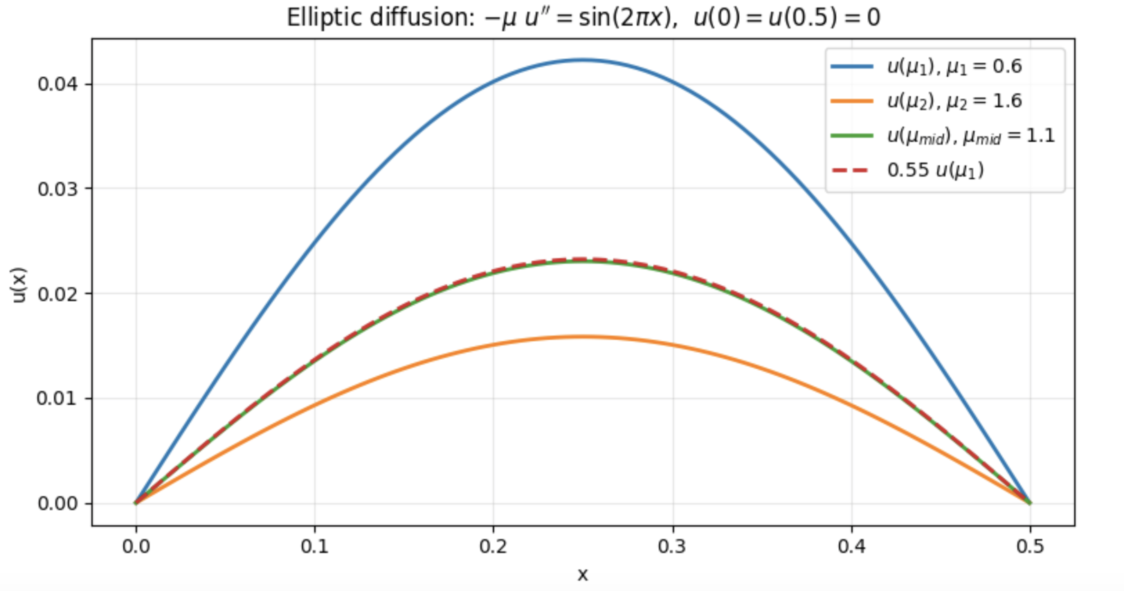

Figure 1: Solution for $\mu_1$ and $\mu_2$ and solution for $\mu_{mid}=\frac{\mu_1+\mu_2}{2}$ and its aproximation from $\mu_1$: $0.55 \ u(\mu_1)$.

This first example (Figure 1) illustrates an obvious case in which the solution for any parameter in $\mathcal{G} \subset \mathbb{R}$ can be determined from a single parameter value.

Now, if we consider another parameterized problem, the question then is:

How many parameter values are needed to efficiently approximate the solution of any other parameter value in $\mathcal{G}$?

More precisely, we seek an approximation of $u(\mu)$ from linear combination of solutions associated with suitably chosen paraemter values.

$$\boxed{ u(\mu) \simeq \sum_{i=1}^N \alpha_i(\mu) u(\mu_i)}$$

Example 2 (or counterexample)

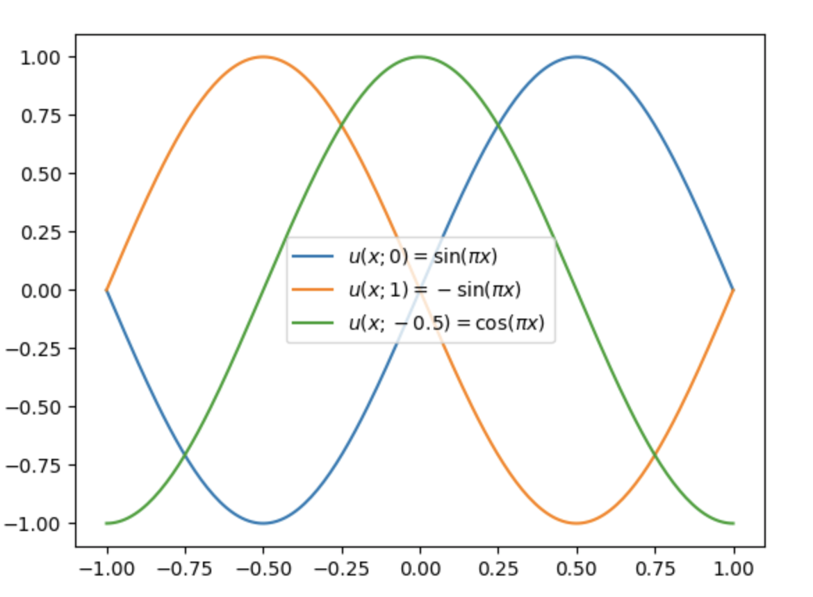
Let us consider the function

$$ u(x; \ \mu) = \mathrm{sin}(\pi (x-\mu)) $$

Let $\mu_1 = 0$. Then:

$$u(x; \ \mu_1) =\mathrm{sin}(\pi x)$$

Let $\mu_2 = 1$. Then

$$ \begin{align*} u(x; \ \mu_2) &=\mathrm{sin}(\pi (x-1))\\ &=-\mathrm{sin}(\pi x) \end{align*} $$

We plot these two solutions in Figure 2. We observe that the two solutions are shifted relative to each other. If we consider a solution lying between these two (as in Figure 2) and attempt to approximate it by a linear combination of the solutions associated with $\mu_1$ and $\mu_2$ (Figure 3), we observe that the result is not satisfactory. Thus, many parameters are required in that case (the linear combination may increase or decrease the amplitude, but it cannot account for the shift).

Figure 2: Solution for $\mu_1$ and $\mu_2$

Figure 3: Approximation of $u(\mu_3)$ by linear combination of $u(\mu_1)$ and $u(\mu_2)$

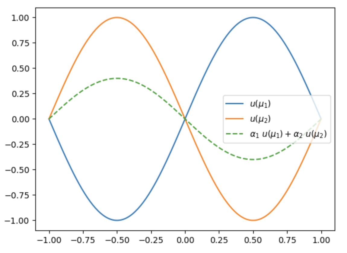
More generally, transport- or convection-dominated effects are difficult to approximate using RBM.

With RBM, we look for a solution on a manifold which implies a reduction of complexity. This complexity reduction relies on the notion of the Kolmogorov n-width. It is linked to the concept of solution manifold, which is the set of all solutions, to the parameterized problem (2) under a parameter variation. If we consider the discretized solution, computed with a High-Fidelity (HF) code (i.e. the solver of our classical discretization method), the solution manifold is denoted $\mathcal{S}_h$

$$\begin{equation} \mathcal{S}_h=\{u_h(\mu)\in V_h| \ \mu \in \mathcal{G}\}. \end{equation}$$

RBM can be successful if the Kolmogorov n-width is small, which means that the solution manifold $\mathcal{S}_h$ (3) might be approximated by a finite set of well-chosen solutions.

We define the Kolmogorov N-width of $\mathcal{S}_h$ as follows:

If $\mathcal{S}_h$ is a subset of a Banach space $V$, and $V_N$ a generic N-dimensional subspace of $V$, then the deviation between $\mathcal{S}_h$ and $V_N$ is

$$\begin{equation} E(\mathcal{S}_h;V_N)=\underset{x\in \mathcal{S}_h}{\sup}(\underset{y \in V_N}{\inf} \lVert| {x-y}\rVert|_{V}). \end{equation}$$

Then the Kolmogorov N-width of $\mathcal{S}_h$ in $V$ is

$$\begin{equation} d_N(\mathcal{S}_h,V)= \underset{V_N}{\inf} \{ E(\mathcal{S}_h;V_N); \mathrm{ V_N \ is\ a\ \textrm{ N-dimensional}\ subspace\ of \ } V \}. \end{equation}$$

It measures how close our vector space $V_N$ is to the optimal space in terms of the uniform projection error of the solutions onto this space.

Finding the optimal space $V_N$ can be difficult, or even impossible. Our goal is therefore to approximate it as closely as possible by selecting suitable parameter values and constructing, from the associated well-chosen solutions, called snapshots, an $n$-dimensional space with a small Kolmogorov N-width, with $N$ kept as small as possible.

RBM aim at approximating any solution belonging to $\mathcal{S}_h$ with a small number of basis functions $N$. The optimal reduced space $V_N$ may not be found but there exists two main algorithms to find reduced spaces that can approximate well any solution of $\mathcal{S}_h$: the Proper Orthogonal Decomposition (POD) or greedy algorithms. In general, greedy algorithms are more efficient if they are combined with aposteriori errors (weak greedy). In both cases, the set of basis functions is derived from HF solutions for several well chosen parameter values, $\{u_h(\mu_1),\dots,u_h(\mu_N)\}$, called snapshots.

Visit this notebook for a comparison between POD/Greedy/SVD/rSVD offline algorithms.

The small Kolmogorov n-width (5) implies that the manifold $\mathcal{S}_h$ can be approximated with very few RB functions, provided that the parameters are chosen for the RB construction properly. Thanks to that, RBM enable HF real-time simulations and widely reduce the computational costs, with speedups that can reach several orders of magnitude.

The main idea of reduced basis methods (RBMs) is to decompose the overall procedure into two parts. The first one, referred to as the offline stage, is computationally expensive but carried out only once, and consists in constructing $V_N$. The second one, called the online stage, is very fast and consists in computing the reduced coordinates in the basis of $V_N$.

Next