POD-Galerkin
The Galerkin-Proper Orthogonal Decomposition (Galerkin-POD) is one of the most popular model reduction techniques for nonlinear partial differential equations. It is based on a Galerkin-type approximation, where the POD basis functions contain information from a solution of the dynamical system at pre-specified instances, so-called snapshots.
Offline
A POD procedure (in other words, SVD or PCA)
Online
A reduced problem with a Galerkin projection to solve
Codes:
Details:
A model problem
Let us introduce the stationary Navier-Stokes equation in the 2D lid driven cavity problem with non-homogeneous Dirichlet boundary conditions on the upper side, homogeneous Dirichlet (no-slip) boundary conditions on the remaining sides, where the domain $\Omega$ is the unit square. The 2D steady Navier-stokes equation writes:
$$ \begin{align*} &-\nu \Delta u + (u \cdot \nabla) u + \nabla p =0, \textrm{ in } \Omega,\\ & \nabla. u=0, \textrm{ in } \Omega,\\ & (u_1,u_2)=(1,0), \textrm{ on } \Omega_{up}:=\partial \Omega \cap \{y=1\},\\ & (u_1,u_2)=(0,0), \textrm{ on } \partial \Omega \backslash \Omega_{up}, \end{align*} $$where
$u=(u_1,u_2) \in V:=H^1_{d,0}(\Omega)^2=\{u \in~H^1(\Omega)^2, u=~(0,0) \textrm{ on } \partial \Omega \backslash \Omega_{up}, \ \textrm{and } u=(1,0) \textrm{ on } \Omega_{up} \}$ represents the velocity of the incompressible fluid, $ p \in L^2(\Omega)$ its pressure, and $\nu=\frac{1}{Re}$ where $Re$ is the Reynolds parameter. Here, the Reynolds number is our parameter of interest ($\mu=Re$).
We impose the average of the pressure $\int_{\Omega} p$ to be equal to $0$ to ensure its uniqueness.
The problem 2D lid driven cavity problem can be rewritten into its variational form:
$$ \begin{equation*} \textrm{ Find }(u,p) \in V \times L^2_0(\Omega)),\textrm{ such that} \end{equation*} $$$$ \begin{align} & a(u,v;\nu)+b(v,p)=0,\forall v \in H^1_0(\Omega)^2 \\ & b(u,q)=0,\forall q \in L^2_0(\Omega) \end{align} $$$$\begin{equation*} a(u,v;\nu)=(u \cdot \nabla u,v)+\nu(\nabla v,\nabla u), \textrm{ and } b(u,q)=-(\nabla \cdot u, q). \end{equation*}$$We assume the problem is well posed and that it satisfies the so-called inf sup condition (or LBB).
With FEM, there exist several types of stable elements. A classical one is the Taylor-Hood element, where basis functions of degree $k$ are used for the pressure and basis functions of degree $k+1$ are employed for the velocities. Thus, we use Taylor-Hood $\mathbb{P}_2-\mathbb{P}_1$ elements to solve the problem in the python notebook. The velocity is approximated with $\mathbb{P}_2$ FE, whereas the pressure is approximated with $\mathbb{P}_1$ FE.
For the nonlinearity we adopt a fixed-point iteration scheme, and after multiplying by test functions $q$ and $v$ (resp. for pressure and velocity), which in variational form reads:
$$\begin{equation} \nu (\nabla u^k, \nabla v) + ((u^{k-1} \cdot \nabla) u^k,v) - (p^k, \nabla \cdot v) - (q, \nabla \cdot u^k) + 10^{-10} (p^k, q) =0, \textrm{in } \Omega, \end{equation}$$where $u^{k-1}$ is the previous step solution, and we iterate until a threshold is reached (until $\|u^{k}-u^{k-1}\| < \varepsilon $).
With the Taylor-Hood elements, we obtain the system $\mathbf{K} \mathbf{x} =\mathbf{f}$ to solve where $\mathbf{K}= \begin{pmatrix} \mathbf{A} & -\mathbf{B}^T\\ -\mathbf{B} & 10^{-10} \mathbf{C} \end{pmatrix}$, $\mathbf{x}$ stands for the tuple velocity-pressure $(u_1^k,u_2^k,p^k)$, and where the assembled matrix $\mathbf{A}$ corresponds to the bilinear part $ \nu (\nabla u^k, \nabla v) + ((u^{k-1} \cdot \nabla) u^k),v) $, the matrix $ B$ to the bilinear part $( p^k ,\nabla \cdot v)$ and $\mathbf{C}$ is the mass matrix applied to the pressure variable ($(\cdot,\cdot)$ represents either the $L^2$ inner-product onto the velocity space or onto the pressure space).
In order to use the POD-Galerkin method, in a general context, we need an affine decomposition with respects to the parameter $\nu$. From the algorithm point of view, the parameter-independent terms are computed offline, making the online computation faster. If this assumption is not fulfilled, we resort to EIM.
The POD has been applied to a wide range of applications (turbulence, image processing applications, analysis of signal, in data compression, optimal control,…).
We detail its offline part, and the online projection stage. There are several forms of POD (classical POD, Snapshots POD, spectral POD,…), and here we consider the Snapshots POD algorithm for the offline part. To sum up, the algorithm is as follows:
- In the offline part, the RB is built with several instances (called the snapshots) of the problem, for several well chosen parameter values. This step consists, first, in forming the snapshots correlation matrix and in retrieving its eigenvalues and its eigenvectors (as in an Singular Value Decomposition). Then, the reduced basis (RB) functions are constructed by linear combinations of the first $N$ eigenvectors with the snapshots, after having sorted the eigenvalues in descending order.
- The online part consists in solving the reduced problem which uses the RB and a Galerkin projection for a new parameter $\mu \in \mathcal{G}$. At the end of the algorithm, a reduced solution for $\mu$ is created.
OFFLINE STAGE
For one parameterized problem, the POD approximation consists in determining a basis of proper orthogonal modes which represents the best the solutions. The goal is to build a reduced space $V_N \subset V$ of dimension $N$, so that the solution $u(x,\mu)$ can be very quickly approximated by its projection onto $V_N$:
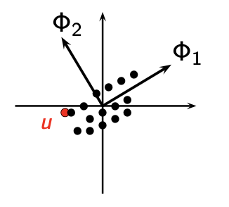
$$u(x; \mu) \simeq \sum_{k=1}^N a_k(\mu) \Phi_k(x)$$with $(\Phi_k)_{k=1,\dots,N}$ an orthonormal basis of $V_N$, and the coefficients $a_k(\mu) = (u_h(\mu),\Phi_k)_V$.
Let us consider $\mu$ as a random variable and $u$ centered ($\mathbb{E}_{\mu}[u] =0$), and let $(\cdot,\cdot)=(\cdot,\cdot)_V$.
POD is analogous to PCA in statistics, as it aims to identify the axes that best represent the data (see Figure 1).
More precisely, we aim to minimize the reduced-basis approximation error on average:
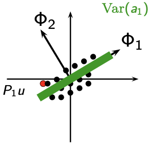
$$ \boxed{\underset{\left\|\Phi_i\right\|=1}{\mathrm{min}}\ \mathbb{E} \left[\left\|u- \sum_{k=1}^N a_k(\mu) \ \Phi_k\right\|^2 \right],} $$or in an equivalent manner, we aim to maximize the variance of the coefficients (Figure 2):
$$ \begin{equation} \underset{\left\|\Phi_i\right\|=1}{\mathrm{max}} \mathbb{E}[|(u,\Phi_i)|^2]. \end{equation} $$Indeed, Koenig-Huygens formula writes $ Var(a_1)=\mathbb{E}[a_1^2] - (\mathbb{E}[a_1])^2 = \mathbb{E}[a_1^2] $.
We now detail why this maximization problem is equivalent to solving an eigenvalue problem.
To avoid overloading the text with notation, let us consider that $V$ is a real Hilbert space.
See here for the complex Hilbert space
Let $\overline{\cdot}$ denotes the average over the observations. In analogy with the real setting, we end up with the following constrained optimization problem:
Find $\Phi$ such that
$$\begin{equation} \displaystyle \max_{\psi \in L^2(\Omega \times \mathcal{G})} \frac{\overline{|(u,\psi)|^2}}{\lVert{\psi}\rVert^2}=\frac{\overline{|(u,\Phi)|^2}}{\lVert{\Phi}\rVert^2}, \end{equation}$$with $\lVert{\Phi}\rVert^2=1$ (To simplify the notation, $\lVert{\cdot}\rVert_{L^2(\Omega \times \mathcal{G})}$ is written $\lVert{\cdot}\rVert$). We can show that equation (1) is equivalent to an eigenvalue problem.
Indeed, to find the maximum, we use the Lagrangian of (1) $J[\phi]=\overline{|(u,\phi)|^2}-\lambda(\rVert{\phi}\rVert^2-1) $ and a variation $\psi$, such that:
$$\begin{equation} \frac{d}{d\delta}J[\phi+\delta \psi]_{|\delta=0}=0. \end{equation}$$$$ \begin{align*} \frac{d}{d\delta}J[\phi+\delta\psi]_{|\delta=0}&=\frac{d}{d\delta}[\overline{|(u,\phi+\delta\psi)|^2}-\lambda(\lVert{\phi+\delta\psi}\rVert^2-1]_{|\delta=0},\nonumber \\ &=\frac{d}{d\delta}[\overline{(u,\phi+\delta\psi)(\phi+\delta\psi,u)}-\lambda(\phi+\delta\psi,\phi+\delta\psi)]_{|\delta=0},\nonumber \\ &=\overline{(u,\phi)(\psi,u)+(u,\psi)(\phi,u)}-\lambda((\phi,\psi)+(\phi,\psi)),\nonumber \\ &=2Re[\overline{(u,\psi)(\phi,u)}-\lambda(\phi,\psi)]. \end{align*}$$Thus, permuting mean operations and integrations entails:
$$\begin{align*} \frac{d}{d\delta}J[\phi+\delta\psi]_{|\delta=0}&=2\overline{(\int_{X}u(X)\cdot\psi^*(X)\ dX) (\int_{X}\phi(X')\cdot u^*(X')\ dX')}-2\lambda\int_{X}\phi(X)\cdot\psi^*(X)dX, \nonumber\\ &=2\int_{X}[\int_{X}\overline{u(X)\cdot u^*(X')}\phi(X')dX'-\lambda\phi(X)]\cdot\psi^*(X)dX. \end{align*} $$$\psi$ being an arbitrary variation, and because $u$ are not functions here but vectors, the auto-correlation function is replaced by a tensor product matrix, and we obtain from (5)
$$\begin{equation} \int_{X}\overline{u(X) \otimes u^*(X')}\phi(X')dX'=\lambda \phi(X). \end{equation}$$$$\begin{equation*} R(X,X')=\overline{u(X) \otimes u^*(X')} \end{equation*}$$is the correlation tensor in two points. The classical method consists in replacing the mean $\overline{(\cdot)}$ by an average over the parameter of interest. On the contrary, the snapshots POD replaces the mean as a space mean over the spatial domain $\Omega$.
We obtain the following eigenvalue problem:
$$\begin{equation} \mathcal{R}\phi=\lambda\phi. \end{equation}$$$\mathcal{R}$ is a positive linear compact self-adjoint operator on $L^2(\Omega \times \mathcal{G})$. Indeed,
$$\begin{align} (\mathcal{R}\Phi,\Phi)&=\int_X\int_X R(X,X')\Phi(X')dX' \cdot \Phi^*(X)dX, \nonumber \\ &=\int_X\int_{X} \overline{u(X) \otimes u^*(X')}\Phi(X')dX' \cdot\Phi^*(X)dX, \nonumber \\ &=\overline{\int_{X} u(X) \cdot \Phi^*(X) dX \int_{X} u^*(X')\cdot\Phi(X')dX'}, \nonumber \\ &=\overline{\lVert{(u,\Phi)}\rVert^2} \geq 0. \nonumber \end{align}$$In the same manner, we can show that $(\mathcal{R}\Phi,\Psi)=(\Phi,\mathcal{R}\Psi)$ for all $(\Psi,\Phi)\in [L^2(\Omega \times \mathcal{G})]^2$.
Therefore, the spectral theory can be applied and guarantees that the maximization problem (1) has one unique solution equal to the largest eigenvalue of the problem (7). which can be reformulate as a Fredholm integral equation
$$\begin{equation} \int_{X}R(X,X')\Phi_n(X')dX'=\lambda^n \Phi_n(X), \end{equation}$$As a consequence, there exists a countable family of solutions $\{\lambda^n,\Phi_n\}$ to equation (8) which represent the eigenvalues and the POD eigenvectors of order $n=1,\dots,+\infty$. The $(\Phi_n)_{n=1,\dots,+\infty}$ are orthogonal (and we can normalize them), and the eigenvalues are all positives.
Proof [eigenvalue problem in real Hilbert space]
We start with the Lagrangian of (1):
$$ J[\Phi_i]=\mathbb{E}[|(u,\Phi_i)|^2] - \lambda(\|\Phi_i\|^2 -1). $$We consider its Gâteaux derivative at $\Phi_i$ in a direction $\Psi$:
$J[\Phi_i+\delta \Psi]=$ $\mathbb{E}[|(u , \Phi_i+\delta \Psi)|^2]$ $-\lambda(\|\Phi_i+\delta \Psi\|^2 -1)$.
Since we want to maximise $J$, we have $\left.\frac{d}{d\delta}J[\Phi_i+\delta\Psi]\right|_{\delta=0}=0.$
$(u,\Phi_i + \delta \Psi)=(u,\Phi_i)+\delta(u,\Psi)$. So,
$(u,\Phi_i+\delta\Psi)^2=(u,\Phi_i)^2+2\delta(u,\Phi_i)(u,\Psi)+O(\delta^2)$
and with average:
$\mathbb{E}[(u,\Phi_i+\delta\Psi)^2]=\mathbb{E}[(u,\Phi_i)^2]+2\delta\mathbb{E}[(u,\Phi_i)(u,\Psi)]+O(\delta^2)$
Thus, $\boxed{\left.\frac{d}{d\delta}\mathbb{E}[(u,\Phi_i+\delta\Psi)^2]\right|_{\delta=0}=2\mathbb{E}[(u,\Phi_i)(u,\Psi)]}$$(\Phi_i+\delta\Psi,\Phi_i+\delta\Psi)=(\Phi_i,\Phi_i)+2\delta(\Phi_i,\Psi)+O(\delta^2)$, so $\boxed{\left.\frac{d}{d\delta}(\Phi_i+\delta\Psi,\Phi_i+\delta\Psi)\right|_{\delta=0}=2(\Phi_i,\Psi)}$
Let $C$ be such that $(C\Phi_i,\Psi)=\mathbb{E}[(u,\Phi_i)(u,\Psi)]$. Then
$$ (C \Phi_i,\Psi)= \lambda (\Phi_i,\Psi), \forall \Psi \in V_N.$$
Since this is true for all $\Psi$, we obtain:
One can easily prove that $C$ is a positive linear compact self-adjoint operator: the problem is well-posed.
Well-posed eigenvalue problem
Compactness of $C$
Assume that \(u \in L^2(\mathcal{G};V)\).
The operator \(C:V\to V\) is defined by
$$C\Phi := \mathbb{E}\big[(u,\Phi)\,u\big],\qquad \Phi\in V.$$We first note that \(C\) is well defined and bounded. Indeed, for every \(\Phi \in V\),
\[ \|(u,\Phi)\,u\|_V \le |(u,\Phi)|\,\|u\|_V \le \|u\|_V\,\|\Phi\|_V\,\|u\|_V = \|\Phi\|_V\,\|u\|_V^2. \]Since \(u\in L^2(\mathcal{G};V)\), we have \(\mathbb{E}\|u\|_V^2<\infty\), hence
$$ \mathbb{E}\big[\|(u,\Phi)\,u\|_V\big] \le \|\Phi\|_V\,\mathbb{E}\|u\|_V^2<\infty. $$\[ \|C\Phi\|_V= \left\|\mathbb{E}\big[(u,\Phi)\,u\big]\right\|_V \le \mathbb{E}\big[\|(u,\Phi)\,u\|_V\big] \le \|\Phi\|_V\,\mathbb{E}\|u\|_V^2, \]so \(C\) is well defined and bounded.
Since \(C\) is also clearly linear, it is continuous and it is positive since
\[ (C \Phi,\Phi)= \mathbb{E}[(u,\Phi)^2] \geq 0. \]We now prove the compactness of \(C\).
Since \(u\in L^2(\mathcal{G};V)\), there exists a sequence \((u_m)_{m\ge 1}\) of finite range such that
\[ u_m \to u \qquad \text{in } L^2(\mathcal{G};V). \]For each \(m\), we define the operator \(C_m:V\to V\) by
$$ C_m\Phi := \mathbb{E}\big[(u_m,\Phi)\,u_m\big]. $$- Each \(C_m\) is finite-rank.
Indeed, since \(u_m\) takes only finitely many values, there exist measurable sets \(A_1,\dots,A_{N_m}\) and vectors \(v_1,\dots,v_{N_m}\in V\) such that
$$ u_m(\omega)=\sum_{j=1}^{N_m}\mathbf{1}_{A_j}(\omega)\,v_j. $$Hence $(u_m,\Phi)_V\,u_m=\sum_{j=1}^{N_m}\mathbf{1}_{A_j}(v_j,\Phi)_V\,v_j.$
Taking the average yields $C_m\Phi=\sum_{j=1}^{N_m}\mathbb{P}(A_j)\,(v_j,\Phi)_V\,v_j.$
Thus $C_m\Phi\in \mathrm{span}\{v_1,\dots,v_{N_m}\} \ \ \forall \Phi\in V$, so $C_m$ has finite rank, and in particular, $C_m$ is compact.
- To prove the compactness of $C$, it suffices to show that $C_m \to C$.
Let $\Phi\in V$ with $\|\Phi\|_V\le 1$. Then
Taking norms and using the triangle inequality,
$$ \|(C-C_m)\Phi\|_V\le\mathbb{E}\big[|(u-u_m,\Phi)|\,\|u\|_V\big]+\mathbb{E}\big[|(u_m,\Phi)|\,\|u-u_m\|_V\big]. $$Since \(\|\Phi\|_V\le 1\),
$$ \|(C-C_m)\Phi\|_V\le\mathbb{E}\big[\|u-u_m\|_V\,\|u\|_V\big]+\mathbb{E}\big[\|u_m\|_V\,\|u-u_m\|_V\big]. $$Applying Cauchy–Schwarz in \(L^2(\mathcal{G})\), we get
$$\mathbb{E}\big[\|u-u_m\|_V\,\|u\|_V\big]\le\|u-u_m\|_{L^2(\mathcal{G};V)}\,\|u\|_{L^2(\mathcal{G};V)},$$and $\mathbb{E}\big[\|u_m\|_V\,\|u-u_m\|_V\big]\le\|u_m\|_{L^2(\mathcal{G};V)}\,\|u-u_m\|_{L^2(\mathcal{G};V)}.$
Hence, taking the supremum over all $\Phi$ such that $\|\Phi\|_V\le 1$, we obtain
$$ \|C-C_m\|_{\mathcal{L}(V)}\le\|u-u_m\|_{L^2(\mathcal{G};V)}\big(\|u\|_{L^2(\mathcal{G};V)}+\|u_m\|_{L^2(\mathcal{G};V)}\big). $$Since \(u_m\to u\) in \(L^2(\mathcal{G};V)\), we have
$\|u-u_m\|_{L^2(\mathcal{G};V)}\to 0,$ and the sequence $(\|u_m\|_{L^2(\mathcal{G};V)})_m$ is bounded. Therefore,
$$\|C-C_m\|_{\mathcal{L}(V)}\to 0.$$Since the limit of compact operators is compact, the operator $C$ is compact, and therefore we can apply the spectral theorem.
Spectral theorem (Compact Self-Adjoint Operator) Let $V$ be a separable Hilbert space and let $C : V \to V$ be a compact, positive, self-adjoint operator. Then there exists a Hilbert basis $\{\Phi_n\}_{n \in \mathbb{N}}$ of $V$ and a sequence of real numbers $(\lambda_n)_{n \in \mathbb{N}}\geq 0$ such that, for all $n \in \mathbb{N}$, $C \Phi_n = \lambda_n \Phi_n$ Moreover, $\lim_{n \to \infty} \lambda_n = 0 .$
The eigenvalue problem is well posed and has a countable family of solutions $\{\lambda_i,\Phi_i\}$.
Solving (1) corresponds to finding the largest eigenvalue $\lambda_1$.
Indeed, with the constraint $\|\Phi_i\|=1$,
Therefore, with the POD, we retrieve the first $N$ largest eigenvalues, and the POD energy error, to choose $N$ and to measure the accuracy of the POD, reads
$$ \begin{equation}\boxed{\mathbb{E}[\|u-P_N u \|^2] = \sum_{k>N} \mathbb{E}[a_k^2]= \sum_{k>N} \lambda_k}. \end{equation} $$We conclude this paragraph by introducing $R$ the spatial continuous covariance operator, defined by $R(x,x'):= \mathbb{E}[u(x) u (x')].$ We remark that
$$\boxed{\mathbb{E}[\underbrace{(u,\Phi)}_a u]=\lambda \Phi, \textrm{ i. e. }C\Phi = \lambda \Phi \Leftrightarrow \int_{\Omega} R(x,x') \ \Phi(x') dx'= \lambda \Phi(x).}$$We have described above the classical POD, where the kernel is the spatial continuous covariance operator, even though in practice the term POD most often refers to the snapshot POD, where one consider a snapshot (= parameter) correlation matrix.
From classical POD to snapshot POD
We now approximate the average in the spatial covariance operator by a sum over some parameters in a training set $\mathcal{G}_{train} \subset \mathcal{G}$:
$$R(x,x')= \mathbb{E}[u(x) u (x')] \simeq \frac{1}{N_{train}} \sum_{k=1}^{N_{train}} u(x, \mu_k) u(x', \mu_k). $$so (2) $\Leftrightarrow \frac{1}{N_{train}}$$\sum_{k=1}^{N_{train}}$ $u(x, \mu_k)$$\underbrace{\int_{\Omega} u(x', \mu_k) \Phi(x') dx'}_{a_k=(u(\mu_k),\Phi)}= \lambda \Phi(x),$
$\textrm{ Therefore } \Phi(x)=$$\sum_{k=1}^{N_{train}}$$ \alpha_k $ $u(x, \mu_k)$,
where, $a_k=(u(\mu_k), \Phi)=(u(\mu_k),\sum_{j=1}^{N_{train}} \alpha_j u(\mu_j))=\sum_{j=1}^{N_{train}} \alpha_j \underbrace{(u(\mu_k), u(\mu_j))}_{\mathbf{C}_{k,j}}$
So the problem (2) becomes
$ \frac1{N_{train}} $$\sum_{k=1}^{N_{train}}$ $u(x, \mu_k)$$\sum_{j=1}^{N_{train}} \alpha_j \mathbf{C}_{k,j} =\lambda $$\sum_{k=1}^{N_{train}}$ $\alpha_k$ $u(x, \mu_k)$,
where $\mathbf{C}$ is the snapshot correlation matrix.
It then gives for one $k=i$
$$\boxed{ \frac1{N_{train}} \sum_{j=1}^{N_{train}} \mathbf{C}_{i,j}\alpha_j =\lambda \alpha_i.}$$Thus, $\mathbf{C}\alpha= N_{train} \lambda \alpha=\lambda' \alpha$: the eigenvalues of the spatial covariance operator or the snapshot correlation matrix are the same (up to a factor $N_{train}$).
So, in the snapshot POD, we solve
$$ \begin{equation} \mathbf{C}\alpha= \lambda' \alpha \end{equation} $$When $N_{\mathrm{train}}$ is much smaller than the dimension of the discrete space, the resulting computational savings are substantial compared to the classical POD.
Snapshot POD algorithm
We impose $(\alpha_n)$ orthonormal.
Let $S=[u_1,\dots,u_{N_{train}}] \in \mathbb{R}^{\mathcal{N} \times N_{train}}.$
Then $\Phi=S \alpha$, and $\|\Phi\|_{L^2(\Omega)}^2=(S\alpha,S\alpha)_{L^2(\Omega)}=\alpha^T \underbrace{S^T S}_{\mathbf{C}} \alpha$
But $(3)$ implies that $ \|\Phi\|_{L^2(\Omega)}^2=\lambda' \alpha^T \alpha=\lambda'$
Hence to normalize the basis functions we write $ \tilde{\Phi}(x)=\frac1{\sqrt{\lambda'}} \sum_{k=1}^{N_{train}} \alpha_k u(x,\mu_k).$
In what follows, we keep the same notations and replace $\tilde{\Phi}$ by $\Phi$ and $\lambda'$ by $\lambda$.
POD algorithm
- Collect snapshots \(u(\cdot,\mu_i)\), for \(i=1,\dots,N_{\text{train}}\)
- Assemble the snapshot matrix \(S\)
- Compute the correlation matrix
$C = S^T S \quad \text{or} \quad C = S^T M_V S$ where $M_V$ is the matrix associated to the scalar product on $V$. - Solve the eigenvalue problem $ C \alpha_i = \lambda_i \alpha_i, \qquad i=1,\dots,N_{\text{train}}$
- Sort the eigenvalues
- Retain the first $N$ eigenvalues/eigenvectors
- Build the POD modes $ \Phi_i = \frac{1}{\sqrt{\lambda_i}} S \alpha_i, \qquad i=1,\dots,N$
How to choose \(N\)?
$$ \mathrm{RIC}(N)=1 - \frac{\sum_{k=1}^{N} \lambda_k}{\sum_{k=1}^{N_{\text{train}}} \lambda_k},$$and we choose $N$ such that \(\mathrm{RIC}(N)\) is close to $0$ (RIC$(N) \simeq \varepsilon$ for a prescribed tolerance).
For the eigenvalues that are too small, we can use a further step which consists in a Gram-Schmidt procedure to ensure the basis orthonormality:
$$\begin{equation*} \Phi_i=\Phi_i-\sum_{j=1}^{i-1} (\Phi_i,\Phi_j)\Phi_j.\end{equation*}$$ONLINE STAGE (Galerkin projection)
We detail now the online stage applied to our model problem. During the last step of the offline stage, the reduced basis $(\Phi_i)_{i=1,...,N} \in \mathbf{V}_N \subset \mathbf{V}_{div}=\{v \in \mathbf{V}_h: \ \nabla.v=0 \}$ is generated. To predict the velocity $u$ for a new parameter $\mu=\nu$, a standard method consists in using a Galerkin projection onto this RB.
This stage is much faster than the execution of HF codes. The assembling reduced order matrices can be computed offline, and therefore only the new reduced problem with these (already computed) matrices needs to be solved during the online phase.
Having reduced bases $(\Phi_i)_{i=1,\dots,N}$ for the velocity and $(\Psi_i)_{i=1,\dots,N}$ for the pressure, we may complete the offline part by assembling the new matrices of our problem:
Instead of using $(u,p)$ in our scheme as before
$$\begin{equation*} \nu (\nabla u, \nabla v) + ((u \cdot \nabla) u,v) - (p, \nabla \cdot v) - (q, \nabla \cdot u) + 10^{-10} (p, q) =0, \textrm{in } \Omega, \end{equation*}$$we replace them by $(\overline{u}+ \sum_{j=1}^N \alpha^k_j \Phi_j,\overline{p} + \sum_{j=1}^N \beta^k_j \Psi_j)$ and $(v,q)$ by $(\Phi_i,\Psi_i)$. We use the POD on the fluctuations to enhance the role of the snapshot correlation matrix. Thus, we get:
$$\begin{align*} & \nu (\nabla \overline{u}, \nabla \Phi_i) + \nu ( \sum_{j=1}^N \alpha^k_j \nabla \Phi_j, \nabla \Phi_i)\\ & \quad \quad \quad + (\overline{u} \cdot \nabla \overline{u},\Phi_i) + (\overline{u} \cdot \sum_{j=1}^N \alpha^k_j \nabla \Phi_j,\Phi_i) + (\sum_{j=1}^N \alpha^{k}_j \Phi_j \cdot \nabla \overline{u},\Phi_i) + (\sum_{r=1}^N \alpha^{k-1}_r \Phi_r \cdot \sum_{j=1}^N \alpha^k_j \nabla \Phi_j,\Phi_i) \\ & \quad \quad \quad - (\overline{p}, \nabla \cdot \Phi_i) - (\sum_{j=1}^N \beta^k_j \Psi_j, \nabla \cdot \Phi_i)- (\Psi_i, \nabla \cdot \overline{u}) - (\Psi_i, \sum_{j=1}^N \alpha^k_j \nabla \cdot \Phi_j) + 10^{-10} (\overline{p}, \Psi_i) + 10^{-10} (\sum_{j=1}^N \beta^k_j \Psi_j, \Psi_i) =0, \textrm{in } \Omega. \end{align*}$$Since $\nabla \cdot u^k=0$, the reduced basis functions $(\Phi_i)_{i=1,\dots,N}$ belongs to $V_N \subset V_{div}:=\{v \in V, \nabla \cdot v=0\}$ and $(\Psi_i)_{i=1,\dots,N}$ is of average equal to $0$. Therefore it gives
$$\begin{equation*} \nu (\nabla \overline{u}, \nabla \Phi_i) + \nu \sum_{j=1}^N \alpha^k_j ( \nabla \Phi_j, \nabla \Phi_i)+(\overline{u} \cdot \nabla \overline{u},\Phi_i) + \sum_{j=1}^N \alpha^k_j (\overline{u} \cdot \nabla \Phi_j,\Phi_i) + \sum_{j=1}^N \alpha^{k}_j ( \Phi_j \cdot \nabla \overline{u},\Phi_i) + \sum_{j=1}^N \sum_{r=1}^N \alpha^k_j \alpha^{k-1}_r (\Phi_r \cdot \nabla \Phi_j,\Phi_i) =0, \textrm{in } \Omega. \end{equation*}$$We remark that we do not need to generate the reduced basis for the pressure, and that we obtain three kind of terms:
- the ones that do not depend on the coefficients $\alpha$,
- the ones that depend on the coefficients $\alpha^k$,
- and one term that depends on the $\alpha^k$ and on the $\alpha^{k-1}$.
Therefore, we shall regroup these terms such that we get:
$$\begin{equation} \mathcal{A}_i + \sum_{j=1}^N \mathcal{B}_{ij} \alpha^k_j + \sum_{j=1}^N \sum_{r=1}^N \mathcal{C}_{ijr} \alpha^k_j \alpha^{k-1}_r =0, \end{equation}$$where
$$\begin{equation*} \mathcal{A}_i = \nu \underbrace{(\nabla \overline{u}, \nabla \Phi_i)}_{A1} + \underbrace{(\overline{u} \cdot \nabla \overline{u},\Phi_i)}_{A2}, \textrm { and } \mathcal{B}_{ij} = \nu \underbrace{ ( \nabla \Phi_j, \nabla \Phi_i)}_{B1} + \underbrace{(\overline{u} \cdot \nabla \Phi_j,\Phi_i)}_{B2} + \underbrace{( \Phi_j \cdot \nabla \overline{u},\Phi_i)}_{B3} \textrm{ and }\mathcal{C}_{ijr} =( \Phi_r \cdot \nabla \Phi_j,\Phi_i). \end{equation*}$$We compute offline the matrices $A1, \ A2,\ B1, \ B2, \ B3 \ $ and $\mathcal{C}$.
During the online stage, we just set the new parameter of interest $\nu$, and compute $\mathcal{A}$, and $\mathcal{B}$ from the offline computed matrices, and with the notations
$$\begin{equation*} M_{ij}=\mathcal{B}_{ij}+\sum_{k=1}^N \mathcal{C}_{ijl} \alpha^{k-1}_l \quad \quad \textrm{and} \quad \quad b_i=\mathcal{A}_i, \end{equation*}$$the coefficients $(\alpha_{j}^k)_{j=1,...,N}$ at iteration $k$ are obtained by solving the reduced problem:
$$\begin{equation*} \mathbf{M} \alpha^k=\mathbf{b}, \end{equation*}$$where $\mathbf{M} \in \mathbb{R}^{N\times N}$ does not depend on $\mathcal{N}$ the degrees of freedom!
Finally, we iterate on the residual $\lVert{{\alpha^k}-{\alpha^{k-1}}}\rVert$ until reaching a small treshold in order to obtain ${\alpha}$, and the approximation is given by
$$\begin{equation*} u_h(\nu)\simeq u_{h,m}+\sum_{j=1}^N \alpha_j \Phi_j. \end{equation*}$$